Use #2: Out of Pipeline • demcrit

If you do not have access to the raw data used in our article, you can still apply the key demcrit functions to your own, similarly structured dataset. In this vignette, we show how to do that using a small reproducible example.

Before you start, make sure you have a local installation of the demcrit R package. If not, see the package overview for installation instructions.

Setup

Start by loading the required packages:

library(demcrit)
library(gt) # for nicely formatted tables
library(tidyverse) |> suppressPackageStartupMessages() # For data wrangling

Data Simulation

Because the original dataset cannot be shared, we will simulate a similar dataset using built-in functions:

set.seed(87542) # for reproducibility
data <- simulate_pdd_data()

You can inspect the default parameters used in this simulation via:

prepare_defaults()
#> $Mu
#>   FAQ  MMSE  MoCA sMoCA 
#>  4.05 26.69 24.07 11.26 
#> 
#> $Sigma
#>             FAQ      MMSE      MoCA     sMoCA
#> FAQ   23.912100 -2.279718 -4.594644 -3.483636
#> MMSE  -2.279718  4.928400  4.867128  3.284712
#> MoCA  -4.594644  4.867128 12.110400  9.058440
#> sMoCA -3.483636  3.284712  9.058440  7.507600
#> 
#> $cens
#>       [,1] [,2]
#> FAQ      0   30
#> MMSE     0   30
#> MoCA     0   30
#> sMoCA    0   16
#> 
#> $crits
#>           IADL IADL_thres cognition cognition_thres
#> MMSE (1)   FAQ          7      MMSE              26
#> MMSE (2)  FAQ9          1      MMSE              26
#> MoCA (1)   FAQ          7      MoCA              26
#> MoCA (2)  FAQ9          1      MoCA              26
#> sMoCA (1)  FAQ          7     sMoCA              13
#> sMoCA (2) FAQ9          1     sMoCA              13

This produces the following example dataset:

#> # A tibble: 1,218 × 8
#>    id       FAQ  MMSE  MoCA sMoCA  FAQ9 type      PDD
#>    <glue> <dbl> <dbl> <dbl> <dbl> <dbl> <chr>     <lgl>
#>  1 s1         6    29    25    12     2 MMSE (1)  FALSE
#>  2 s1         6    29    25    12     2 MMSE (2)  FALSE
#>  3 s1         6    29    25    12     2 MoCA (1)  FALSE
#>  4 s1         6    29    25    12     2 MoCA (2)  TRUE
#>  5 s1         6    29    25    12     2 sMoCA (1) FALSE
#>  6 s1         6    29    25    12     2 sMoCA (2) TRUE
#>  7 s2        12    24    21     9     3 MMSE (1)  TRUE
#>  8 s2        12    24    21     9     3 MMSE (2)  TRUE
#>  9 s2        12    24    21     9     3 MoCA (1)  TRUE
#> 10 s2        12    24    21     9     3 MoCA (2)  TRUE
#> # ℹ 1,208 more rows

Key variables include:

id – patient identifier
type – diagnostic algorithm used
PDD – diagnosis result for each patient–algorithm pair

For more details about how the data are generated, see:

help("simulate_pdd_data") # details on the data generation algorithm
help("prepare_defaults") # details on parameter defaults

Dementia Rates

To compute dementia (PDD) rates, we first prepare a specification of diagnostic algorithms and variable mappings. Then, we pass these to the summarise_rates() function:

# Extract default parameters:
pars <- prepare_defaults()

# Define algorithm specifications:
algos <- with(pars, {data.frame(
  type = rownames(crits),
  glob = crits$cognition, glob_t = crits$cognition_thres,
  iadl = crits$IADL, iadl_t = crits$IADL_thres,
  atte = "", atte_t = NA,
  exec = "", exec_t = NA,
  memo = "", memo_t = NA,
  cons = "", cons_t = NA,
  lang = "", lang_t = NA
)})

# Define variable names:
vars <- data.frame(
  name = c(unique(algos$glob), unique(algos$iadl)),
  label = c(unique(algos$glob), unique(algos$iadl)),
  type = "continuous"
)

# Compute PDD rates:
rates <- summarise_rates(
  list(PDD = data, algorithms = algos),
  vars = vars,
  plot = FALSE # Setting plot to FALSE bacause it is calibrated the data from the study..
)

# Format results:
tab1 <- rates$table |>
  select(type, Global, IADL, N, Rate) |>
  gt_apa_table() |>
  cols_label(
    type ~ "Algorithm",
    Global ~ "Cognitive deficit",
    IADL ~ "IADL deficit"
  )

Table 1: An example table showing simulated PDD rates.

Algorithm	Cognitive deficit	IADL deficit	N	Rate

MMSE (1)	MMSE < 26	FAQ > 7	203	17 (8.37%)
MMSE (2)	MMSE < 26	FAQ9 > 1	203	48 (23.65%)
MoCA (1)	MoCA < 26	FAQ > 7	203	29 (14.29%)
MoCA (2)	MoCA < 26	FAQ9 > 1	203	85 (41.87%)
sMoCA (1)	sMoCA < 13	FAQ > 7	203	31 (15.27%)
sMoCA (2)	sMoCA < 13	FAQ9 > 1	203	91 (44.83%)

Pairwise Concordance

Next, we can compute pairwise concordance statistics across algorithms:

concs <- describe_concordance(list(PDD = data, algorithms = algos))

For details about the resulting object, see:

help("describe_concordance")
help("concords") # describes the concordance statistics table

We can visualize concordance matrices for several metrics:

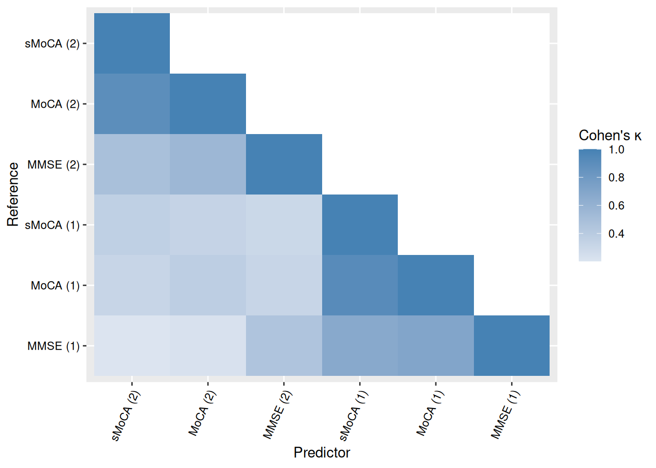
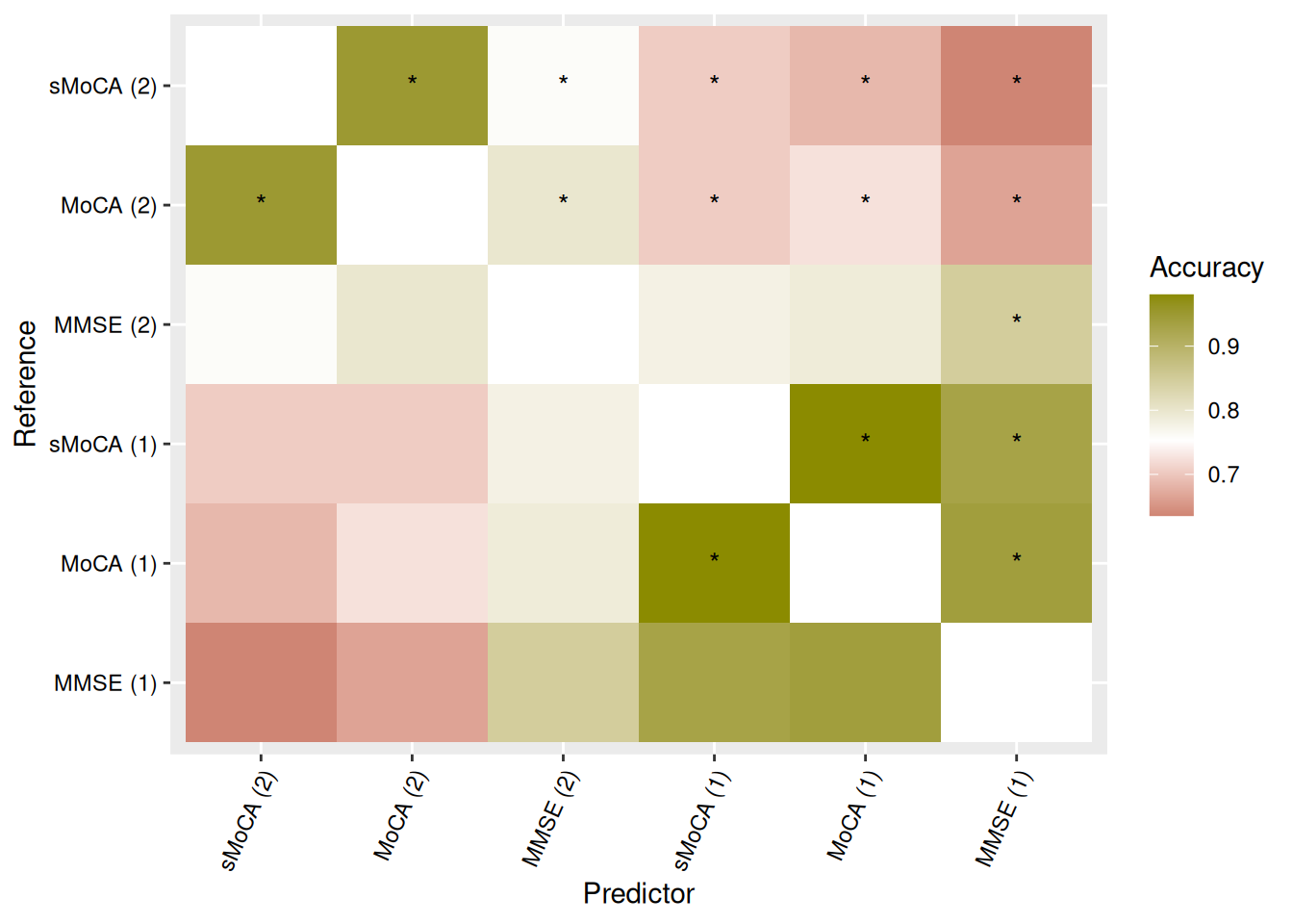
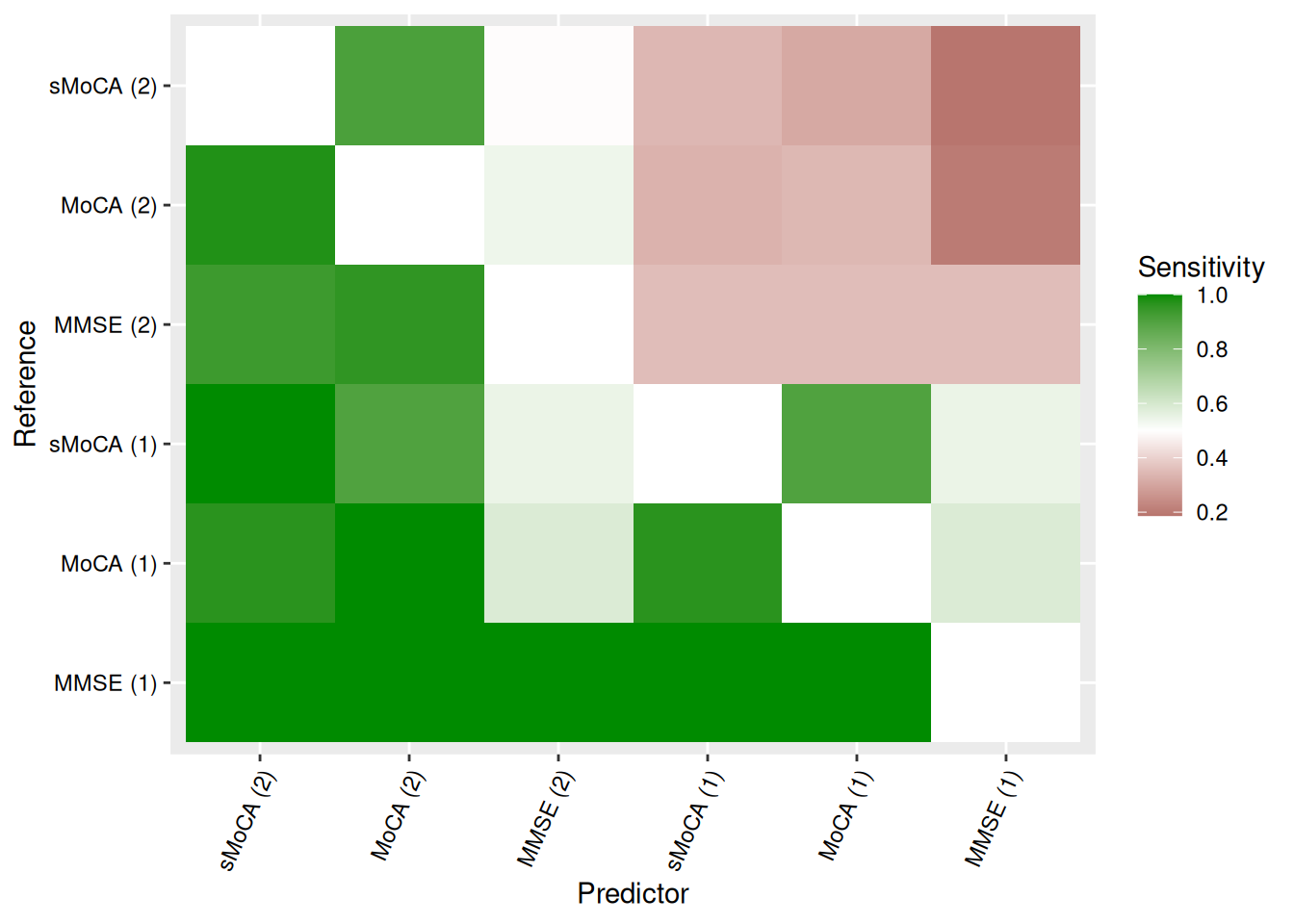
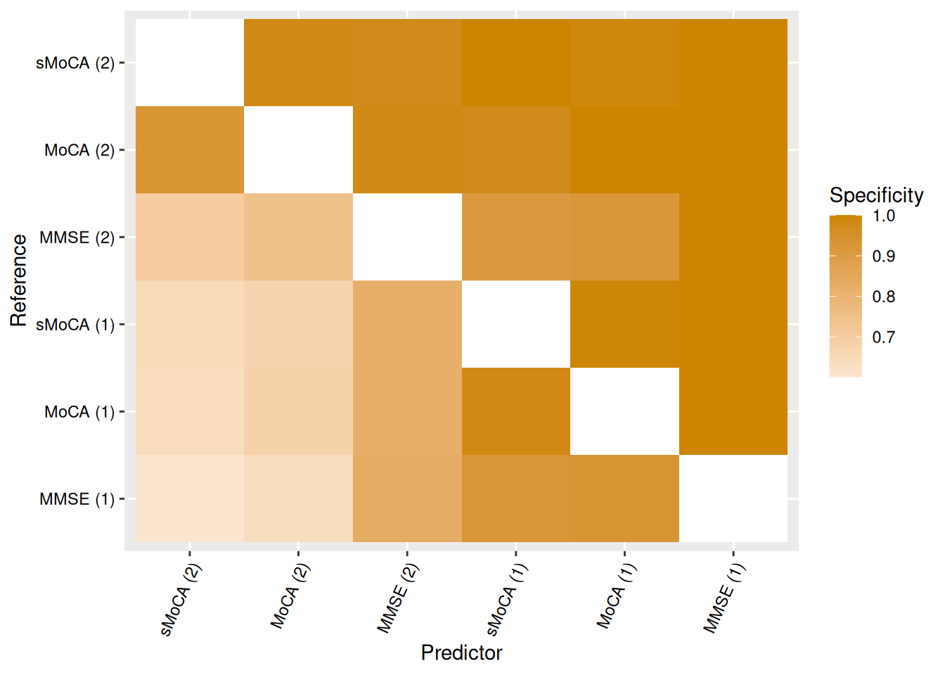
Alternatively, we can extract specific concordance statistics and present them in a table. Table Table 2 shows one such example, with algorithms sorted by raw accuracy in predicting MoCA (1).

tab2 <- concs$table |>
  filter(reference == "MoCA (1)") |>
  filter(reference != predictor) |>
  arrange(desc(Accuracy_raw)) |>
  select(predictor, Kappa, Accuracy, NoInformationRate_raw, AccuracyPValue) |>
  mutate(AccuracyPValue = do_summary(AccuracyPValue, 3, "p")) |>
  gt_apa_table() |>
  fmt_number(decimals = 2) |>
  cols_label(
    predictor ~ "Predictor",
    NoInformationRate_raw ~ "NIR",
    AccuracyPValue ~ "p-value"
  )

Table 2: Example table showing pairwise concordance statistics for five algorithms sorted by raw accuracy in predicting MoCA (1). NIR stands for No Information Rate, and p-values correspond to one-sided binomial tests of Accuracy > NIR.

Predictor	Kappa	Accuracy	NIR	p-value

sMoCA (1)	0.92 [0.85, 1.00]	0.98 [0.95, 0.99]	0.86	< .001
MMSE (1)	0.71 [0.56, 0.86]	0.94 [0.90, 0.97]	0.86	< .001
MMSE (2)	0.32 [0.17, 0.47]	0.79 [0.73, 0.84]	0.86	.997
MoCA (2)	0.38 [0.27, 0.48]	0.72 [0.66, 0.78]	0.86	1.000
sMoCA (2)	0.32 [0.22, 0.42]	0.68 [0.62, 0.75]	0.86	1.000